Monte Carlo integration

Monte Carlo is the simplest of all collocation methods. It consist of the following steps:

1. Generate (pseudo-)random samples \(Q_1, ..., Q_N\).

2. Evaluate model solver \(U_1=u(Q_1), ..., U_N=u(Q_N)\) for each sample.

3. Use empirical metrics to assess statistics on the evaluations.

This was the approached introduced in problem formulation, and we shall go through it again, but in a bit more details, and leveraging some of the features introduced in the section quasi_random_samples.

Generating samples

The samples that shall be used in Monte Carlo must be assumed to behave as if drawn from the probability distribution of the model parameters on want to model. In the case of problem formulation, the samples drawn was random. Here we shall replace the random samples with variance reduced samples from the following three schemes:

• Sobol

• Antithetic variate

• Halton

We start by generating samples from the distribution of interest:

from problem_formulation import joint

joint

J(Normal(mu=1.5, sigma=0.2), Uniform(lower=0.1, upper=0.2))

Then we generate samples from the three schemes:

sobol_samples = joint.sample(10000, rule="sobol")
antithetic_samples = joint.sample(10000, antithetic=True, seed=1234)
halton_samples = joint.sample(10000, rule="halton")

from matplotlib import pyplot

pyplot.rc("figure", figsize=[16, 4])

pyplot.subplot(131)
pyplot.scatter(*sobol_samples[:, :1000])
pyplot.title("sobol")

pyplot.subplot(132)
pyplot.scatter(*antithetic_samples[:, :1000])
pyplot.title("antithetic variates")

pyplot.subplot(133)
pyplot.scatter(*halton_samples[:, :1000])
pyplot.title("halton")


pyplot.show()

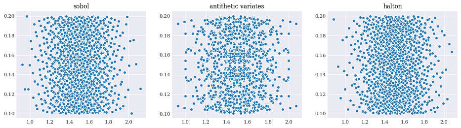
From the three plots above it is easy to see both how the Sobol sequence have more structure, and the antithetic variate have observable symmetries.

Evaluating model solver

Like in the case of problem formulation again, evaluation is straight forward:

from problem_formulation import model_solver, coordinates
import numpy

sobol_evals = numpy.array([
    model_solver(sample) for sample in sobol_samples.T])

antithetic_evals = numpy.array([
    model_solver(sample) for sample in antithetic_samples.T])

halton_evals = numpy.array([
    model_solver(sample) for sample in halton_samples.T])

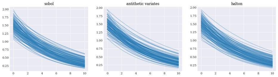
pyplot.subplot(131)
pyplot.plot(coordinates, sobol_evals[:100].T, alpha=0.3)
pyplot.title("sobol")

pyplot.subplot(132)
pyplot.plot(coordinates, antithetic_evals[:100].T, alpha=0.3)
pyplot.title("antithetic variate")

pyplot.subplot(133)
pyplot.plot(coordinates, halton_evals[:100].T, alpha=0.3)
pyplot.title("halton")

pyplot.show()

Error analysis

Having a good estimate on the statistical properties allows us to asses the properties of the uncertainty in the model. However, it does not allow us to assess the accuracy of the methods used. To do that we need to compare the statistical metrics with their analytical counterparts. To do so, we use the reference analytical solution and error function as defined in problem formulation.

from problem_formulation import error_in_mean, indices, eps_mean

eps_sobol_mean = [error_in_mean(
    numpy.mean(sobol_evals[:idx], 0)) for idx in indices]

eps_antithetic_mean = [error_in_mean(
    numpy.mean(antithetic_evals[:idx], 0)) for idx in indices]

eps_halton_mean = [error_in_mean(
    numpy.mean(halton_evals[:idx], 0)) for idx in indices]

pyplot.rc("figure", figsize=[6, 4])

pyplot.semilogy(indices, eps_mean, "r", label="random")
pyplot.semilogy(indices, eps_sobol_mean, "-", label="sobol")
pyplot.semilogy(indices, eps_antithetic_mean, ":", label="antithetic")
pyplot.semilogy(indices, eps_halton_mean, "--", label="halton")

pyplot.legend()
pyplot.show()

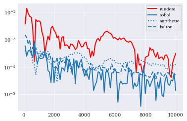
Here we see that for our little problem, all new schemes outperforms classical random samples with Sobol on top, followed by Halton and antithetic variate.

For the error in variance estimation we have:

from problem_formulation import error_in_variance, eps_variance

eps_halton_variance = [error_in_variance(
    numpy.var(halton_evals[:idx], 0)) for idx in indices]

eps_sobol_variance = [error_in_variance(
    numpy.var(sobol_evals[:idx], 0)) for idx in indices]

eps_antithetic_variance = [error_in_variance(
    numpy.var(antithetic_evals[:idx], 0)) for idx in indices]

pyplot.semilogy(indices, eps_variance, "r", label="random")
pyplot.semilogy(indices, eps_sobol_variance, "-", label="sobol")
pyplot.semilogy(indices, eps_antithetic_variance, ":", label="antithetic")
pyplot.semilogy(indices, eps_halton_variance, "--", label="halton")

pyplot.legend()
pyplot.show()

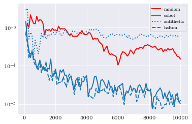
In this case Sobol and Halton er quite comparable as the best performers. Antithetic variate seems to now work out, with performance lower than classical random samples.

Note that the conclusion here is not that antithetic variate don’t work, but rather that it is perhaps not the right tool for this job.