Probability distributions
Probability distribution is the backbone of uncertainty quantification. Creating a probability distribution in chaospy is done by as follows:
[1]:
import chaospy

normal = chaospy.Normal(mu=2, sigma=2)
normal
[1]:
Normal(mu=2, sigma=2)
The distribution have a few methods that the user can used, which has names and syntax very similar to that of scipy.stats. Below some of these methods are demonstrated. For a full overview of the distribution methods, see chaospy.Distribution.
For an overview of available distributions, see then take a look at the collection listed in the reference.
(Pseudo-)random samples
The most important property a random variable has, is to create (pseudo-)random samples. This can be created using chaospy.Distribution.sample():
[2]:
samples = normal.sample(4, seed=1234)
samples
[2]:
array([0.2553786 , 2.62204779, 1.68653451, 3.58083895])
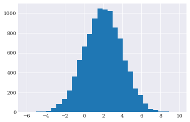
These can be used to create e.g. histograms:
[3]:
from matplotlib import pyplot

pyplot.hist(normal.sample(10000, seed=1234), 30)
pyplot.show()
The input can be both be a integer, but also a sequence of integers. For example:
[4]:
normal.sample([2, 2], seed=1234)
[4]:
array([[0.2553786 , 2.62204779],
       [1.68653451, 3.58083895]])
Random seed
Note that the seed parameters was passed to ensure reproducability. In addition to having this flag, all chaospy distributions respects numpy’s random seed. So the sample generation can also be done as follows:
[5]:
import numpy

numpy.random.seed(1234)
normal.sample(4)
[5]:
array([0.2553786 , 2.62204779, 1.68653451, 3.58083895])
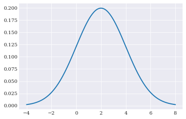
Probability density function
The probability density function, is a function whose value at any given sample in the sample space can be interpreted as providing a relative likelihood that the value of the random variable would equal that sample. This method is available through chaospy.Distribution.pdf():
[6]:
normal.pdf([-2, 0, 2])
[6]:
array([0.02699548, 0.12098536, 0.19947114])
[7]:
q_loc = numpy.linspace(-4, 8, 200)
pyplot.plot(q_loc, normal.pdf(q_loc))
pyplot.show()
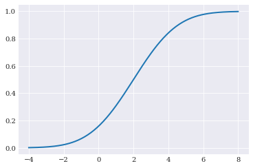
Cumulative probability function
the cumulative distribution function, defines the probability that a random variables is at most the argument value provided. This method is available through chaospy.Distribution.cdf():
[8]:
normal.cdf([-2, 0, 2])
[8]:
array([0.02275013, 0.15865525, 0.5 ])
[9]:
pyplot.plot(q_loc, normal.cdf(q_loc))
pyplot.show()
Statistical moments
The moments of a random variable giving important descriptive information about the variable reduced to single scalars. The raw moments is the building blocks to build these descriptive statistics. The moments are available through chaospy.Distribution.mom():
[10]:
normal.mom([0, 1, 2])
[10]:
array([1., 2., 8.])
Not all random variables have raw moment variables, but for these variables the raw moments are estimated using quadrature integration. This allows for the moments to be available for all distributions. This approximation can explicitly be evoked through chaospy.approximate_moment():
[11]:
chaospy.approximate_moment(normal, [2])
[11]:
8.0
See quadrature integration for more details on how this is done in practice.
Central moments can be accessed through wrapper functions. The four first central moments of our random variable are:
[12]:
(chaospy.E(normal), chaospy.Var(normal),
 chaospy.Skew(normal), chaospy.Kurt(normal))
[12]:
(array(2.), array(4.), array(0.), array(0.))
See descriptive statistics for details on the functions extracting metrics of interest from random variables.
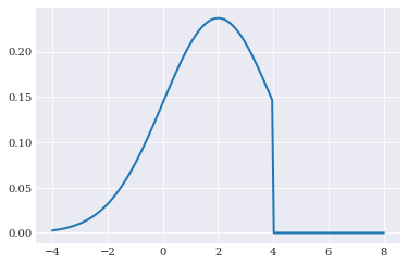
Truncation
In the collection of distributions some distribution are truncated by default. However for those that are not, and that is the majority of distributions, truncation can be invoiced using chaospy.Trunc(). It supports one-sided truncation:
[13]:
normal_trunc = chaospy.Trunc(normal, upper=4)

pyplot.plot(q_loc, normal_trunc.pdf(q_loc))
pyplot.show()
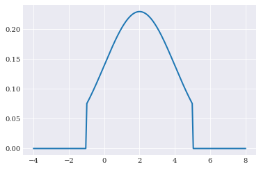
and two-sided truncation:
[14]:
normal_trunc2 = chaospy.Trunc(normal, lower=-1, upper=5)

pyplot.plot(q_loc, normal_trunc2.pdf(q_loc))
pyplot.show()
Multivariate variables
chaospy also supports joint random variables. Some have their own constructors defined in the collection of distributions. But more practical, multivariate variables can be constructed from univariate ones through chaospy.J:
[15]:
normal_gamma = chaospy.J(chaospy.Normal(0, 1), chaospy.Gamma(1))
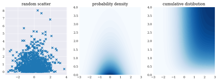
The multivariate variables have the same functionality as the univariate ones, except that inputs and the outputs of the methods chaospy.Distribution.sample, chaospy.Distribution.pdf() and chaospy.Distribution.cdf() assumes an extra axis for dimensions. For example:
[16]:
pyplot.rc("figure", figsize=[12, 4])

pyplot.subplot(131)
pyplot.title("random scatter")
pyplot.scatter(*normal_gamma.sample(1000, seed=1000), marker="x")

pyplot.subplot(132)
pyplot.title("probability density")
grid = numpy.mgrid[-3:3:100j, 0:4:100j]
pyplot.contourf(grid[0], grid[1], normal_gamma.pdf(grid), 50)

pyplot.subplot(133)
pyplot.title("cumulative distibution")
pyplot.contourf(grid[0], grid[1], normal_gamma.cdf(grid), 50)

pyplot.show()
Rosenblatt transformation
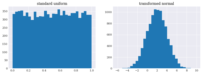
One of the more sure-fire ways to create random variables, is to first generate classical uniform samples and then use a inverse transformation to map the sample to have the desired properties. In one-dimension, this mapping is the inverse of the cumulative distribution function, and is available as chaospy.Distribution.ppf():
[17]:
pyplot.subplot(121)
pyplot.title("standard uniform")
u_samples = chaospy.Uniform(0, 1).sample(10000, seed=1234)
pyplot.hist(u_samples, 30)

pyplot.subplot(122)
pyplot.title("transformed normal")
q_samples = normal.inv(u_samples)
pyplot.hist(q_samples, 30)

pyplot.show()
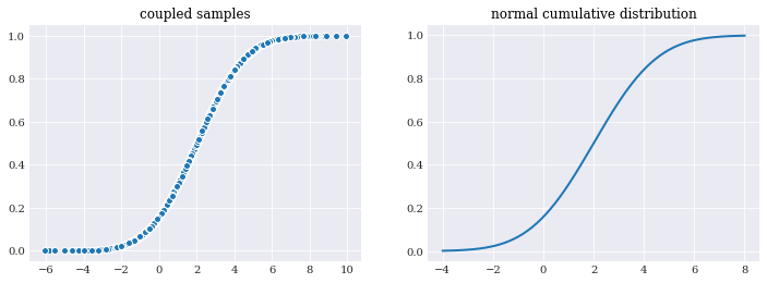
Note that u_samples and q_samples here consist of independently identical distributed samples, the joint set (u_samples, q_samples) are not. In fact, they are highly dependent by following the line of the normal cumulative distribution function shape:
[18]:
pyplot.subplot(121)
pyplot.title("coupled samples")
pyplot.scatter(q_samples, u_samples)

pyplot.subplot(122)
pyplot.title("normal cumulative distribution")
pyplot.plot(q_loc, normal.cdf(q_loc))

pyplot.show()
This idea also generalizes to the multivariate case. There the mapping function is called an inverse Rosenblatt transformation \(T^{-1}\), and is defined in terms of conditional distribution functions:
And likewise a forward Rosenblatt transformation is defined as:
These functions can be used to map samples from standard multivariate uniform distribution to a distribution of interest, and vise-versa.
In chaospy these methods are available through chaospy.Distribution.inv() and chaospy.Distribution.fwd():
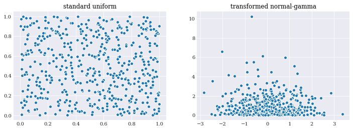
[19]:
pyplot.subplot(121)
pyplot.title("standard uniform")
uu_samples = chaospy.Uniform(0, 1).sample((2, 500), seed=1234)
pyplot.scatter(*uu_samples)

pyplot.subplot(122)
pyplot.title("transformed normal-gamma")
qq_samples = normal_gamma.inv(uu_samples)
pyplot.scatter(*qq_samples)

pyplot.show()
User-defined distributions
The collection of distributions contains a lot of distributions, but if one needs something custom, chaospy allows for the construction of user-defined distributions through chaospy.UserDistribution. These can be constructed by providing three functions: cumulative distribution function, a lower bounds function, and a upper bounds function. As an illustrative example, let us recreate the uniform
distribution:
[20]:
def cdf(x_loc, lo, up):
    """Cumulative distribution function."""
    return (x_loc-lo)/(up-lo)
[21]:
def lower(lo, up):
    """Lower bounds function."""
    return lo
[22]:
def upper(lo, up):
    """Upper bounds function."""
    return up
The user-define distribution takes these functions, and a dictionary with the parameter defaults as part of its initialization:
[23]:
user_distribution = chaospy.UserDistribution(
    cdf=cdf, lower=lower, upper=upper, parameters=dict(lo=-1, up=1))
The distribution can then be used in the same was as any other chaospy.Distribution:
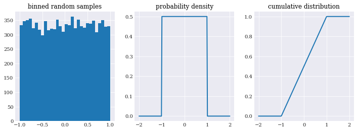
[24]:
pyplot.subplot(131)
pyplot.title("binned random samples")
pyplot.hist(user_distribution.sample(10000), 30)

pyplot.subplot(132)
pyplot.title("probability density")
x_loc = numpy.linspace(-2, 2, 200)
pyplot.plot(x_loc, user_distribution.pdf(x_loc))

pyplot.subplot(133)
pyplot.title("cumulative distribution")
pyplot.plot(x_loc, user_distribution.cdf(x_loc))

pyplot.show()
Alternative, it is possible to define the same distribution using cumulative distribution and point percentile function without the bounds:
[25]:
def ppf(q_loc, lo, up):
    """Point percentile function."""
    return q_loc*(up-lo)+lo


user_distribution = chaospy.UserDistribution(
    cdf=cdf, ppf=ppf, parameters=dict(lo=-1, up=1))
In addition to the required fields, there are a few optional ones. These does not provide new functionality, but allow for increased accuracy and/or lower computational cost for the operations where they are used. These include raw statistical moments which is used by chaospy.Distribution.mom():
[26]:
def mom(k_loc, lo, up):
    """Raw statistical moment."""
    return (up**(k_loc+1)-lo**(k_loc+1))/(k_loc+1)/(up-lo)
And three terms recurrence coefficients which is used by the method chaospy.Distribution.ttr() to pass analytically to Stieltjes’ method:
[27]:
def ttr(k_loc, lo, up):
    """Three terms recurrence."""
    return 0.5*up+0.5*lo, k_loc**2/(4*k_loc**2-1)*lo**2
What these coefficients are and why they are important are discussed in the section orthogonal polynomials.