Quadrature integration

Quadrature methods, or numerical integration, is broad class of algorithm for performing integration of any function \(g\) that are defined without requiring an analytical definition. In the scope of chaospy we limit this scope to focus on methods that can be reduced to the following approximation:

\[\int p(q) g(q) dx \approx \sum_{n=1}^N W_n g(Q_n)\]

Here \(p(q)\) is an weight function, which is assumed to be an probability density function, and \(W_n\) and \(Q_n\) are respectively quadrature weights and abscissas used to define the approximation.

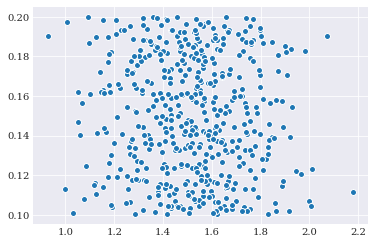
The simplest application of such an approximation is Monte Carlo integration. In Monte Carlo you only need to select \(W_n=1/N\) for all \(n\) and \(Q_n\) to be independent identical distributed samples drawn from the distribution of \(p(q)\). For example:

import numpy
import chaospy

from problem_formulation import joint

joint

J(Normal(mu=1.5, sigma=0.2), Uniform(lower=0.1, upper=0.2))

nodes = joint.sample(500, seed=1234)
weights = numpy.repeat(1/500, 500)

from matplotlib import pyplot

pyplot.scatter(*nodes)
pyplot.show()

Having the nodes and weights, we can now apply the quadrature integration. for a simple example, this might look something like:

from problem_formulation import model_solver

evaluations = numpy.array([model_solver(node) for node in nodes.T])
estimate = numpy.sum(weights*evaluations.T, axis=-1)

How to apply quadrature rules to build model approximations is discussed in more details in pseudo-spectral projection.

Gaussian quadrature

Most integration problems when dealing with polynomial chaos expansion comes with a weight function \(p(x)\) which happens to be the probability density function. Gaussian quadrature creates weights and abscissas that are tailored to be optimal with the inclusion of a weight function. It is therefore not one method, but a collection of methods, each tailored to different probability density functions.

In chaospy Gaussian quadrature is a functionality attached to each probability distribution. This means that instead of explicitly supporting a list of Gaussian quadrature rules, all feasible rules are supported through the capability of the distribution implementation. For common distribution, this means that the quadrature rules are calculated analytically, while others are estimated using numerically stable methods.

Generating optimal Gaussian quadrature in chaospy by passing the flag rule="gaussian" to the chaospy.generate_quadrature() function:

gauss_nodes, gauss_weights = chaospy.generate_quadrature(6, joint, rule="gaussian")

pyplot.scatter(*gauss_nodes, s=gauss_weights*1e4)
pyplot.show()

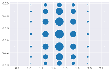
Since joint is bivariate consists of a normal and a uniform distribution, the optimal quadrature here is a tensor product of Gauss-Hermite and Gauss-Legendre quadrature.

Weightless quadrature

Most quadrature rules optimized to a given weight function are part of the Gaussian quadrature family. It does the embedding of the weight function automatically as that is what it is designed for. This is quite convenient in uncertainty quantification as weight functions in the form of probability density functions is almost always assumed. For most other quadrature rules, including a weight function is typically not canonical, however. So for consistency and convenience, chaospy does a small trick and embeds the influence of the weight into the quadrature weights:

\[\int p(q) g(q) dq \approx \sum_i W_i p(Q_i) g(Q_i) = \sum_i W^{*}_i g(Q_i)\]

Here we substitute \(W^{*}=W_i p(Q_i)\). This ensures us that all quadrature rules in chaospy behaves similarly as the Gaussian quadrature rules.

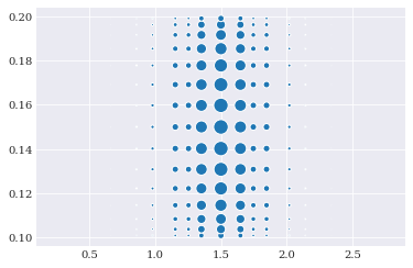
For our bivariate example, we can either choose a single rule for each dimension, or individual rules. Since joint consists of both a normal and a uniform, it makes sense to choose the latter. For example Genz-Keister is know to work well with normal distributions and Clenshaw-Curtis should work well with uniform distributions:

grid_nodes, grid_weights = chaospy.generate_quadrature(
    3, joint, rule=["genz_keister_24", "fejer_2"], growth=True)

pyplot.scatter(*grid_nodes, s=grid_weights*6e3)
pyplot.show()

As a sidenote: Even though embedding the density function into the weights is what is the most convenient think to do in uncertainty quantification, it might not be what is needed always. So if one do not want the embedding, it is possible to retrieve the classical unembedded scheme by replacing the probability density function as the second argument of chaospy.generate_quadrature() with an interval of interest. For example:

interval = (-1, 1)
chaospy.generate_quadrature(4, interval, rule="clenshaw_curtis")

(array([[-1.        , -0.70710678,  0.        ,  0.70710678,  1.        ]]),
 array([0.06666667, 0.53333333, 0.8       , 0.53333333, 0.06666667]))

Also note that for quadrature rules that do require a weighting function, passing an interval instead of an distribution will cause an error:

from pytest import raises

with raises(AssertionError):
    chaospy.generate_quadrature(4, interval, rule="gaussian")

Smolyak sparse-grid

As the number of dimensions increases, the number of nodes and weights quickly grows out of hands, making it unfeasible to use quadrature integration. This is known as the curse of dimensionality, and except for Monte Carlo integration, there is really no way to completely guard against this problem. However there are a few ways to partially mitigate the problem, like Smolyak sparse-grid. Smolyak sparse-grid uses a rule over a combination of different quadrature orders and tailor it together into a new scheme. If the quadrature nodes are more or less nested between the different quadrature orders, as in the same nodes get reused a lot, then the Smolyak method can drastically reduce the quadrature nodes needed.

To use Smolyak sparse-grid in chaospy, just pass the flag sparse=True to the chaospy.generate_quadrature() function. For example:

sparse_nodes, sparse_weights = chaospy.generate_quadrature(
    3, joint, rule=["genz_keister_24", "clenshaw_curtis"], sparse=True)

idx = sparse_weights > 0
pyplot.scatter(*sparse_nodes[:, idx], s=sparse_weights[idx]*2e3)
pyplot.scatter(*sparse_nodes[:, ~idx], s=-sparse_weights[~idx]*2e3, color="grey")
pyplot.show()

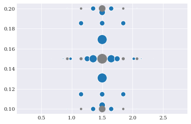
Note that in sparse-grid, the weights are often a mixture of positive and negative values, as illustrated here with the two different colors.

Note here that the flag growth=True was used. This is because a few quadrature rules that are nested only at particular orders. Passing the growth=True flag implies that increasing at the order which is nested. This affects the four quadrature rules: Clenshaw-Curtis, Fejér, Newton-Cotes and grid.