Advanced regression method

The library scikit-learn is a great machine-learning toolkit that provides a large collection of regression methods. By default, chaospy only support traditional least-square regression, but is also designed to work together with the various regression functions provided by scikit-learn.

Because scikit-learn isn’t a required dependency, you might need to install it first with e.g. pip install scikit-learn. When that is done, it should be importable:

import sklearn

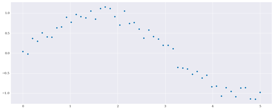
As en example to follow, consider the following artificial case:

import numpy
import chaospy

samples = numpy.linspace(0, 5, 50)
numpy.random.seed(1000)
noise = chaospy.Normal(0, 0.1).sample(50)
evals = numpy.sin(samples) + noise

from matplotlib import pyplot

pyplot.rc("figure", figsize=[15, 6])
pyplot.scatter(samples, evals)
pyplot.show()

Least squares regression

By default, chaospy does not use sklearn (and can be used without sklearn being installed). Instead it uses scipy.linalg.lstsq, which is the ordinary least squares method, the classical regression problem by minimizing the residuals squared.

In practice:

q0 = chaospy.variable()
expansion = chaospy.polynomial([1, q0, q0**2, q0**3])

fitted_polynomial = chaospy.fit_regression(
    expansion, samples, evals)

pyplot.scatter(samples, evals)
pyplot.plot(samples, fitted_polynomial(samples))
pyplot.show()

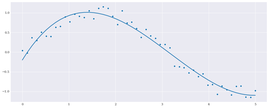
fitted_polynomial.round(4)

polynomial(0.0921*q0**3-0.8798*q0**2+1.9153*q0-0.1982)

Least squares regression is also supported by sklearn. So it is possible to get the same result using the LinearRegression model. For example:

from sklearn.linear_model import LinearRegression

model = LinearRegression(fit_intercept=False)
fitted_polynomial = chaospy.fit_regression(
    expansion, samples, evals, model=model)

pyplot.scatter(samples, evals)
pyplot.plot(samples, fitted_polynomial(samples))
pyplot.show()

fitted_polynomial.round(4)

polynomial(0.0921*q0**3-0.8798*q0**2+1.9153*q0-0.1982)

It is important to note that sklearn often does extra operations that may interfere with the compatibility of chaospy. Here fit_intercept=False ensures that an extra columns isn’t added needlessly. An error will be raised if this is forgotten.

Single variable regression

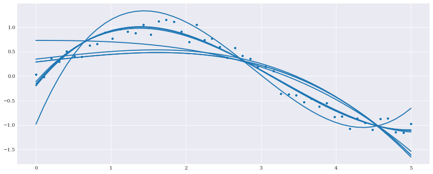
While in most cases least squares regression is sufficient, that is not always the case. For those deviating cases scikit-learn provides a set of alternative methods. Even though chaospy doesn’t differentiate between single dimensional and multi-dimensional responses, scikit-learn do.

The methods that support single dimensional responses are:

• least squares – Simple \(L_2\) regression without any extra features.

• elastic net – \(L_2\) regression with both \(L_1\) and \(L_2\) regularization terms.

• lasso – \(L_2\) regression with an extra \(L_1\) regularization term, and a preference for fewer non-zero terms.

• lasso lars – An implementation of lasso meant for high dimensional data.

• lars – \(L_1\) regression well suited for high dimensional data.

• orthogonal matching pursuit – \(L_2\) regression with enforced number of non-zero terms.

• ridge – \(L_2\) regression with an \(L_2\) regularization term.

• bayesian ridge – Same as ridge, but uses Bayesian probability to let data estimate the complexity parameter.

• auto relevant determination – Same as bayesian ridge, but also favors fewer non-zero terms.

from sklearn import linear_model as lm

kws = {"fit_intercept": False}
univariate_models = {
    "least squares": lm.LinearRegression(**kws),
    "elastic net": lm.ElasticNet(alpha=0.1, **kws),
    "lasso": lm.Lasso(alpha=0.1, **kws),
    "lasso lars": lm.LassoLars(alpha=0.1, **kws),
    "lars": lm.Lars(**kws),
    "orthogonal matching pursuit":
        lm.OrthogonalMatchingPursuit(n_nonzero_coefs=3, **kws),
    "ridge": lm.Ridge(alpha=0.1, **kws),
    "bayesian ridge": lm.BayesianRidge(**kws),
    "auto relevant determination": lm.ARDRegression(**kws),
}

Again, as the polynomials already addresses the constant term, it is important to remember to include fit_intercept=False for each model.

We can then create a fit for each of the univariate models:

for label, model in univariate_models.items():

    fitted_polynomial = chaospy.fit_regression(
        expansion, samples, evals, model=model)
    pyplot.plot(samples, fitted_polynomial(samples))

pyplot.scatter(samples, evals)
pyplot.show()

Multi-variable regression

This part of the tutorial uses the same example as the problem formulation. In other words:

from problem_formulation import (
    model_solver, joint, error_in_mean, error_in_variance)

The methods that support multi-label dimensional responses are:

• least squares – Simple \(L_2\) regression without any extra features.

• elastic net – \(L_2\) regression with both \(L_1\) and \(L_2\) regularization terms.

• lasso – \(L_2\) regression with an extra \(L_1\) regularization term, and a preference for fewer non-zero terms.

• lasso lars – An implementation of lasso meant for high dimensional data.

• orthogonal matching pursuit – \(L_2\) regression with enforced number of non-zero terms.

• ridge – \(L_2\) regression with an \(L_2\) regularization term.

multivariate_models = {
    "least squares": lm.LinearRegression(**kws),
    "elastic net": lm.MultiTaskElasticNet(alpha=0.2, **kws),
    "lasso": lm.MultiTaskLasso(alpha=0.2, **kws),
    "lasso lars": lm.LassoLars(alpha=0.2, **kws),
    "lars": lm.Lars(n_nonzero_coefs=3, **kws),
    "orthogonal matching pursuit": \
        lm.OrthogonalMatchingPursuit(n_nonzero_coefs=3, **kws),
    "ridge": lm.Ridge(alpha=0.2, **kws),
}

To illustrate the difference between the methods, we do the simple error analysis:

import warnings
warnings.filterwarnings("ignore", category=RuntimeWarning)

expansion = chaospy.generate_expansion(2, joint)
samples = joint.sample(50)
evals = numpy.array([model_solver(sample) for sample in samples.T])

for label, model in multivariate_models.items():

    fitted_polynomial, coeffs = chaospy.fit_regression(
        expansion, samples, evals, model=model, retall=True)

    self_evals = fitted_polynomial(*samples)
    error_mean_ = error_in_mean(chaospy.E(fitted_polynomial, joint))
    error_var_ = error_in_variance(chaospy.Var(fitted_polynomial, joint))
    count_non_zero = numpy.sum(numpy.any(coeffs, axis=-1))

    print(f"{label:<30} {error_mean_:.5f} " +
          f"{error_var_:.5f} {count_non_zero}")

least squares                  0.00003 0.00000 6
elastic net                    0.08373 0.02085 2
lasso                          0.01386 0.01541 2
lasso lars                     0.21168 0.02121 1
lars                           0.00061 0.00144 3
orthogonal matching pursuit    0.00114 0.00060 3
ridge                          0.00819 0.00936 6

It is worth noting that as some of the method removes coefficients, it can function at higher polynomial order than the saturate methods.