Gaussian mixture model

Gaussian mixture model (GMM) is a probabilistic model created by averaging multiple Gaussian density functions. It is not uncommon to think of these models as a clustering technique because when a model is fitted, it can be used to backtrack which individual density each samples is created from. However, in chaospy, which first and foremost deals with forward problems, sees GMM as a very flexible class of distributions.

On the most basic level constructing GMM in chaospy can be done from a sequence of means and covariances:

import chaospy

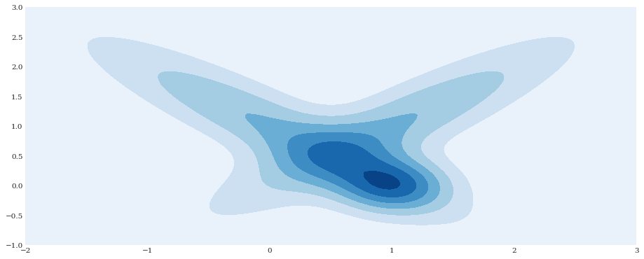
means = ([0, 1], [1, 1], [1, 0])
covariances = ([[1.0, -0.9], [-0.9, 1.0]],
               [[1.0,  0.9], [ 0.9, 1.0]],
               [[0.1,  0.0], [ 0.0, 0.1]])
distribution = chaospy.GaussianMixture(means, covariances)
distribution

GaussianMixture()

import numpy
from matplotlib import pyplot
pyplot.rc("figure", figsize=[15, 6], dpi=75)

xloc, yloc = numpy.mgrid[-2:3:100j, -1:3:100j]
density = distribution.pdf([xloc, yloc])
pyplot.contourf(xloc, yloc, density)

pyplot.show()

Model fitting

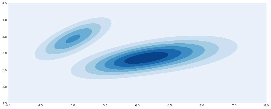
chaospy supports Gaussian mixture model representation, but does not provide an automatic method for constructing them from data. However, this is something for example scikit-learn supports. It is possible to use scikit-learn to fit a model, and use the generated parameters in the chaospy implementation. For example, let us consider the Iris example from scikit-learn’s documentation (“full” implementation in 2-dimensional representation):

from sklearn import datasets, mixture

model = mixture.GaussianMixture(3, random_state=1234)
model.fit(datasets.load_iris().data)

means = model.means_[:, :2]
covariances = model.covariances_[:, :2, :2]
print(means.round(4))
print(covariances.round(4))

[[5.006  3.428 ]
 [6.5464 2.9495]
 [5.9171 2.778 ]]
[[[0.1218 0.0972]
  [0.0972 0.1408]]

 [[0.3874 0.0922]
  [0.0922 0.1104]]

 [[0.2755 0.0966]
  [0.0966 0.0926]]]

distribution = chaospy.GaussianMixture(means, covariances)

xloc, yloc = numpy.mgrid[4:8:100j, 1.5:4.5:100j]
density = distribution.pdf([xloc, yloc])
pyplot.contourf(xloc, yloc, density)

pyplot.show()

Like scikit-learn, chaospy also support higher dimensions, but that would make the visualization harder.

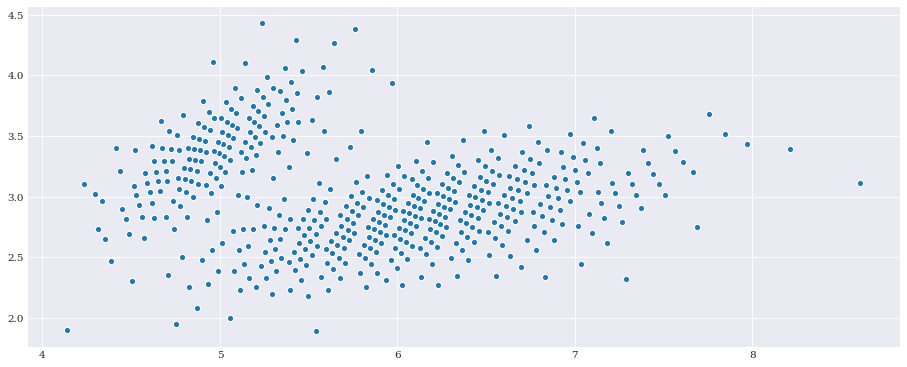
Low discrepancy sequences

chaospy support low-discrepancy sequences through inverse mapping. This support extends to mixture models, making the following possible:

pseudo_samples = distribution.sample(500, rule="additive_recursion")

pyplot.scatter(*pseudo_samples)
pyplot.show()

Chaos expansion

To be able to do point collocation method it requires the user to have access to sampler from the input distribution and orthogonal polynomials with respect to the input distribution. The former is available above, while the latter is available as follows:

expansion = chaospy.generate_expansion(1, distribution, rule="cholesky")

expansion.round(4)

polynomial([1.0, q1-3.0518, 0.2121*q1+q0-6.4705])