Polynomial chaos Kriging

We start by defining a problem. Here we borrow the formulation from uqlab.

import numpy
import chaospy

distribution = chaospy.Uniform(0, 15)
samples = distribution.sample(10, rule="sobol")
evaluations = samples*numpy.sin(samples)
evaluations.round(4)

array([  7.035 , -10.8878,  -2.1434,  -3.4407,   6.9566,   0.4665,
         1.7889,   0.909 ,  -7.9987,  14.0233])

The goal is to create a so called “polynomial chaos kriging” model as defined in the paper with the same name. We are going to do this using the following steps:

• Create a pool of orthogonal polynomials using chaospy.

• Use scikit-learn’s least angular regression model to reduce the pool.

• Use gstools to create an universal Kriging model with the orthogonal polynomials as drift terms.

The result is what is what the paper defines as “sequential polynomial chaos kriging”.

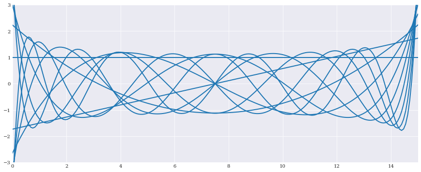
We start by creating a pool of orthonormal polynomials to be selected from:

from matplotlib import pyplot

expansion = chaospy.generate_expansion(9, distribution, normed=True)

t = numpy.linspace(0, 15, 200)
pyplot.rc("figure", figsize=[15, 6])
pyplot.plot(t, expansion(t).T)
pyplot.axis([0, 15, -3, 3])
pyplot.show()

As chaospy does not support least angular regression, we use the scikit-learn implementation. But still pass the job to chaospy to perform the fitting, as it also gives an fitted expansion:

from sklearn.linear_model import LarsCV

lars = LarsCV(fit_intercept=False, max_iter=5)
pce, coeffs = chaospy.fit_regression(
    expansion, samples, evaluations, model=lars, retall=True)
expansion_ = expansion[coeffs != 0]

pce.round(2)

polynomial(0.01*q0**6-0.17*q0**5+1.42*q0**4-5.19*q0**3+5.89*q0**2+4.46*q0-5.32)

Note that the same coefficients can be created from the lars model directly, but that does not yield a fitted expansion:

lars = LarsCV(fit_intercept=False, max_iter=5)
lars.fit(expansion(samples).T, evaluations)
expansion_ = expansion[lars.coef_ != 0]

lars.coef_.round(4)

array([ 0.0000e+00,  0.0000e+00,  0.0000e+00,  5.5500e-01,  0.0000e+00,
       -1.1415e+00, -5.2567e+00, -2.9271e+00,  0.0000e+00,  4.2000e-03])

This resulted in a reduction of the number of polynomials:

print("number of expansion terms total:", len(expansion))
print("number of expansion terms included:", len(expansion_))

number of expansion terms total: 10
number of expansion terms included: 5

With the number of polynomials reduced, we can create our kriging model. In this case we use the excellent gstools library:

import gstools

model = gstools.Gaussian(dim=1, var=1)
pck = gstools.krige.Universal(model, samples, evaluations, list(expansion_))

pck(samples)
assert numpy.allclose(pck.field, evaluations)

For reference, we also create a more traditional universal kriging model with linear drift.

uk = gstools.krige.Universal(model, samples, evaluations, "linear")
uk(samples)
assert numpy.allclose(uk.field, evaluations)

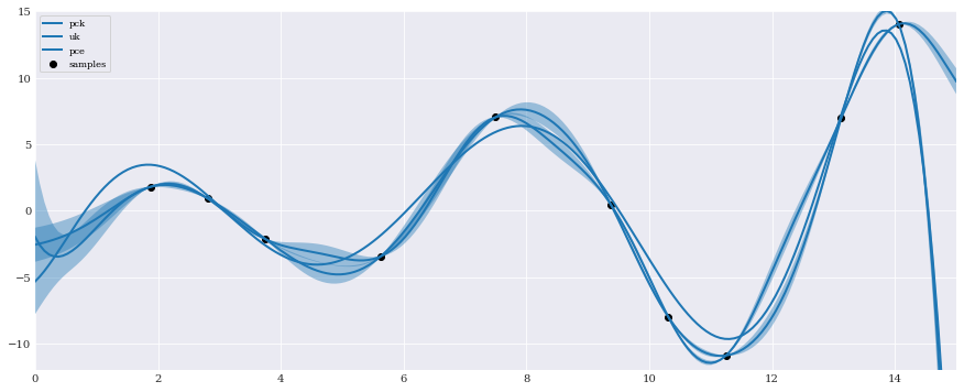
Lastly we visually compare the models by plotting the mean and standard deviations against each other:

pck(t)
mu, sigma = pck.field, numpy.sqrt(pck.krige_var)
pyplot.plot(t, mu, label="pck")
pyplot.fill_between(t, mu-sigma, mu+sigma, alpha=0.4)

uk(t)
mu, sigma = uk.field, numpy.sqrt(uk.krige_var)
pyplot.plot(t, mu, label="uk")
pyplot.fill_between(t, mu-sigma, mu+sigma, alpha=0.4)

pyplot.plot(t, pce(t), label="pce")

pyplot.scatter(samples, evaluations, color="k", label="samples")

pyplot.axis([0, 15, -12, 15])
pyplot.legend(loc="upper left")
pyplot.show()